PyTorch 深度学习实践 | 刘二
Lecture 1 Overview
反向传播 Back Propagation
反向传播就是 求导数?
随着网络层数增多,写解析式太困难了
核心:计算图
目前主流的框架:
-
TensorFlow 一开始使用 Static Graph,现在最新版也是动态
-
PyTorch 使用 Dynamic Graph
学术界大多转到 PyTorch,工业界也有较多用 TensorFlow 的
我tm版本好像太高了,老师用的只是 0.4.0
Lecture 2 线性模型
三步骤:
- DataSet
监督学习:训练集 + 测试集
- Model 选择
- Training
- inferring 推理
Model design
| x | y |
|---|---|
| 1 | 2 |
| 2 | 4 |
| 3 | 6 |
| 4 | ? |
使用线性模型:
Linear Regression
the machine starts with a random guess
where \(\omega\) = random value
把训练集代入,算出\(\hat{y}\)
goal: evaluate model error
Compute Loss
Training Loss
Mean Square Error(MSE) 平均平方误差
Lecture 3 梯度下降算法
Quote
早期机器学习中,我们经常被低维空间的直觉所误导,担心神经网络会像掉进坑里一样陷入“糟糕的局部最优解(Bad Local Minima)”。但现代高维非线性优化的研究证明:在参数量极其庞大的深度神经网络中,真正的敌人不是局部最优点,而是海量的“鞍点(Saddle Points)”以及由它们构成的平原(Plateaus)。
梯度下降
要让随时函数最小,既求出损失函数的梯度
Update:
代码
x_data = [1.0, 2.0, 3.0]
y_data = [2.0, 4.0, 6.0]

w = 1

def forward(x):
    return x * w

def cost(xs, ys):
    cost = 0
    for x, y in zip(xs, ys):
        y_pred = forward(x)
        cost += (y_pred - y) ** 2
    return cost / len(xs)

def gradient(xs, ys):
    grad = 0
    for x, y in zip(xs, ys):
        grad += 2 * x * (forward(x) - y)
    return grad / len(xs)

print("predict(before training):", 4, forward(4))

for epoch in range(100):
    cost_val = cost(x_data, y_data)
    grad_val = gradient(x_data, y_data)
    w -= 0.01 * grad_val
    print("Epoch:", epoch, "w=", w, "loss=", cost_val)

print("predict(after training):", 4, forward(4))
predict(before training): 4 4
Epoch: 0 w= 1.0933333333333333 loss= 4.666666666666667
Epoch: 1 w= 1.1779555555555554 loss= 3.8362074074074086
Epoch: 2 w= 1.2546797037037036 loss= 3.1535329869958857
Epoch: 3 w= 1.3242429313580246 loss= 2.592344272332262
Epoch: 4 w= 1.3873135910979424 loss= 2.1310222071581117
...
Epoch: 95 w= 1.9999177805941268 loss= 3.8376039345125727e-08
Epoch: 96 w= 1.9999254544053418 loss= 3.154680994333735e-08
Epoch: 97 w= 1.9999324119941766 loss= 2.593287985380858e-08
Epoch: 98 w= 1.9999387202080534 loss= 2.131797981222471e-08
Epoch: 99 w= 1.9999444396553017 loss= 1.752432687141379e-08
predict(after training): 4 7.999777758621207
Note
cost 有时候比较波动,用指数加权均值可以让损失函数更平滑
越久远的历史,他的权重呈指数级衰减
实际上在深度学习中梯度下降用的算少的,更多是随机梯度下降
梯度下降(Gradient Descent)是:
随机梯度下降(Stochastic Gradient Descent)则是:
其实就是梯度不再是所有样本的平均损失,而是只抽取一个样本来更新梯度
用每一个样本来更新梯度
不过机器学习是可以并行计算的
但随机梯度下降由于计算依赖前项,无法并行
深度学习里选择折中:Batch-size
每次用一组来梯度下降
Mini-Batch
Lecture 4 反向传播 Back Propagation
?我还以为反向传播已经讲完了呢
matrix-cook-book 电子书有矩阵的求导公式
神经网络中的一层:
\(x \in \mathbb{R}^n, W_1 \in \mathbb{R}^{m \times n}, b \in \mathbb{R}^m\)
两层:\(\hat{y} = W_2(W_1 \cdot X + b_1) + b_2 = W \cdot X + b\)
所以实际上所有层都是线性的话没有意义,就相当于1层
所以要加上一个非线性的变化函数
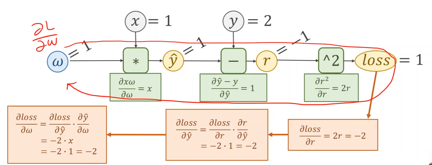
知道 x, y 把\(\frac{\partial{L}}{\partial{\omega}}\)算出来就是反向传播,其实就是链式法则
Tensor in PyTorch
tensor 是 PyTorch 里的基本单位,可以是标量、任意维度矩阵
有两个成员变量:data 和 grad,存储了节点的\(\omega\)的值和 \(\frac{\partial{loss}}{\partial{\omega}}\)
代码
import torch

x_data = [1.0, 2.0, 3.0]
y_data = [2.0, 4.0, 6.0]

w = torch.Tensor([1.0])
w.requires_grad = True
# 由 require_grad=True 的变量参与计算产生的新 Tensor,都会被自动计算 grad_fn,指向生成他的那个运算节点

def forward(x):
    return x * w

def loss(x, y):
    return (forward(x) - y) ** 2

# 每次调用 loss 函数,其中的每个算术运算都对应了 C++ 的Function 子类,这些 Function 记录了怎么向前算,也记录了怎么反向求导,就生成了计算图

print("prediction before training:", 4, forward(4).item())

for epoch in range(100):
    for x, y in zip(x_data, y_data):
        l = loss(x, y)
        l.backward() # 计算 \partial{l} / \partial{w},自动累加到 w.grad里
        print("grad:", x, y, w.grad.item())
        w.data = w.data - 0.01 * w.grad.data
        # 注意是在.data(w.data, w.grad.data)上更新参数,因为他们的.requires_grad==False,也就没有grad_fn,不会被统计进计算图

        w.grad.data.zero_()
        # 清空梯度(这里使用的是SGD 随机梯度下降,所以在每一个样本后都清零)
        # 如果是 Min Batch 梯度下降,则在每个 Batch 后清零
        # "_"代表原地操作

    print("progress:", epoch, l.item())

print("predict after training",  4, forward(4).item())
总结一下流程就是:
- 准备工作,创建张量
- 前向传播(内部隐藏构建计算图)
- 反向传播(自动计算梯度(内部实现好了))
- 更新参数
- 清空梯度(根据使用的梯度下降是哪种,选择是每个样本都清空梯度,还是一个 Batch 清空一次)
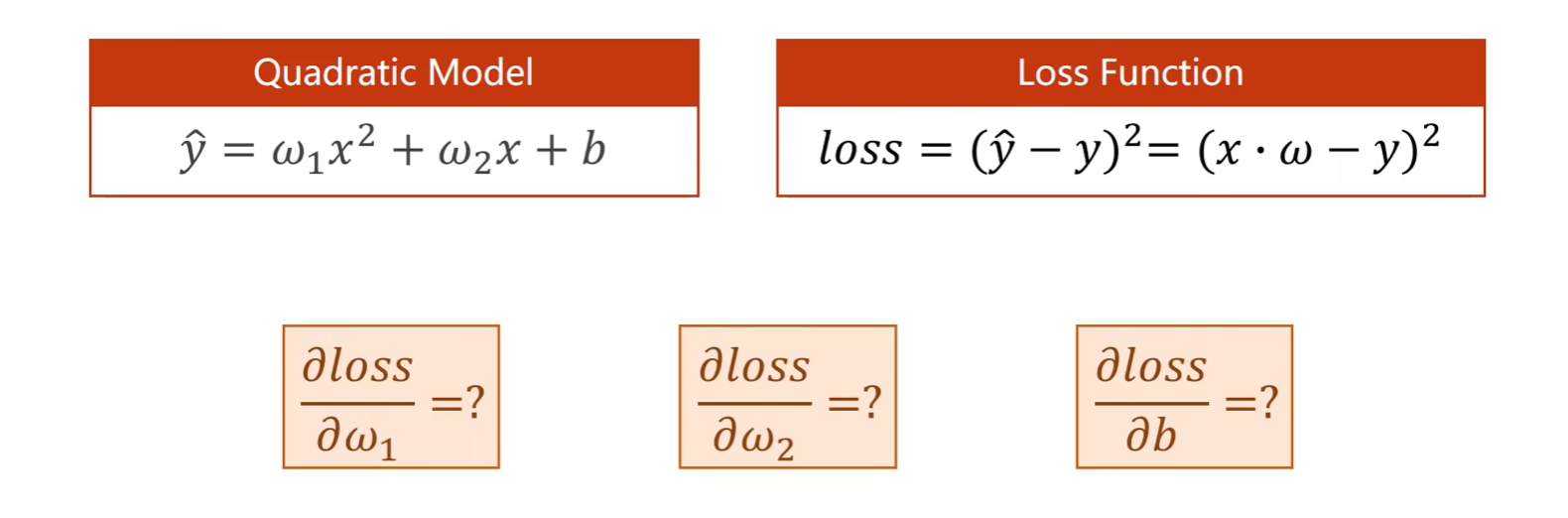
作业
Lecture 5 Linear Regression with Pytorch 用pytorch实现线性回归
回顾
-
forward 正向:算出损失
-
backward 反向:算出梯度
-
然后更新参数
梳理一下框架!
-
prapare dataset
-
design model using class
inherit from nn.Module
-
construct loss and optimizer
using pytorch API
-
Training cycle
forward, backward, update
1. prepare dataset
import torch

x_data = torch.Tensor([[1.0], [2.0], [3.0]])
y_data = torch.Tensor([[2.0], [4.0], [6.0]])
我的理解就是一个batch就是一个矩阵
2. design model
之前没有使用pytorch的时候,我们还要计算如何计算导数
但是使用pytorch我们的工作就转移到构建计算图
构建完了pytorch就自动把梯度计算出来了
关于损失函数
因为之前说的数据里,min_batch都是一个矩阵,所以一个batch计算出的loss也会是一个矩阵:
真正的\(loss\)就要把这个矩阵平均后变成标量
# 创建一个继承于torch.nn.Module的子类
class LinearModel(torch.nn.Module): # nn是neural network
    def __init__(self):
        super(LinearModel, self).__init__()
        self.linear = torch.nn.Linear(1, 1)
        #

    def froward(self, x):
        y_pred = self.linear(x)
        return y_pred

model = LinearModel()
3. Construct Loss and Optimizer
criterion = torch.nn.MSELoss(size_average=False)
# class torch.nn.MSELoss(size_average=True, reduce=True)
# mean squared error
optimizer = torch.optim.SGD(model.parameters(), lr=0.01)
# class torch.optim.SGD(params, lr=<object object>, momentum=0, weight_decay=0, nesterov=False)
# parameters 会检查所有成员,是否需要计算权重
# momentum 冲量
# weight_decay: w^T w
4. training cycle
for epoch in range(100):
    y_pred = model(x_data)
    loss = criterion(y_pred, y_data)
    print(epoch, loss) # 这里打印loss只会调用__str__不会再调用一遍loss,是安全的

    optimizer.zero_grad() # loss调用的时候自动
    loss.backward()
    optimizer.step() # update
等价于我们之前手工更新的过程
import torch

x_data = torch.Tensor([[1.0], [2.0], [3.0]])
y_data = torch.Tensor([[2.0], [4.0], [6.0]])


# 将模型封装成一个类,且要继承自 nn.Module
class LinearModel(torch.nn.Module):
    def __init__(self):
        super(LinearModel, self).__init__() # 简洁写法 super.__init__()
        self.linear = torch.nn.Linear(1, 1)
        '''
        class torch.nn.Linear(in_feature, out_feature, bias=True)
        - in_feature: size of each input sample
        - out_feature: size of each output sample
        - bias: if set to false, the layer will not learn an additive bias. Default: True
        '''
    # forward 函数实现(必须要叫forward)
    def forward(self, x):
        y_pred = self.linear(x)
        # self.linear是一个实例,一个实例能够加括号调用说明这个对象的类或父类实现了__call__()
        # call: y = w x + b

        return y_pred

model = LinearModel()

criterion = torch.nn.MSELoss(size_average=False)

optimizer = torch.optim.SGD(model.parameters(), lr=0.01)
# class torch.optim.SGD(params, lr=<object object>, momentum=0, weight_decay=0, nesterov=False)

for epoch in range(100):
    y_pred = model(x_data)
    loss = criterion(y_pred, y_data)
    print(epoch, loss) # 这里打印loss只会调用__str__不会再调用一遍loss,是安全的

    optimizer.zero_grad() # loss调用的时候自动
    loss.backward()
    optimizer.step() # update

# output weight and bias
print('w = ', model.linear.weight.item())
print('b = ', model.linear.bias.item())

# test model
x_test = torch.Tensor([[4.0]])
y_test = model(x_test)
print('y_pred = ', y_test.data)
pytorch 里提供了很多优化器:
- torch.optim.Adagrad
- torch.optim.Adam
- torch.optim.Adamax
- torch.optim.ASGD
- torch.optim.LBFGS
- torch.optim.RMSprop
- torch.optim.Rprop
- torch.optim.SGD
(pytorch 官网实例)[https://pytorch.org/tutorials/beginner/pytorch_with_examples.html]
Lecture 6 Logistic Regression
分类问题
输出的是 是每一类的概率
下载数据集
因为分类问题输出的是概率,所以输出\(\hat{y}\)的值域为[0, 1]
还有很多别的sigmoid函数(S型函数)
affine model 仿射模型
先前学的简单线性(仿射)变换
Logistic Regression Model
损失函数的变化
线性回归问题中,损失函数是在计算\(\hat{y}\)与y间的几何距离
而二分类问题中,损失函数是交叉熵
\(\hat{y} = P(class = 1), (1-\hat{y}) = P(class = 0)\)
y只有0和1两种输入,\(\hat{y}\)与y越接近,熵越小
Mini-Batch Loss Function for Binary Classification
在上述的基础上,说明mini-batch的损失函数
import torch.nn.functional as F

class LogisticRegressionModel(torch.nn.Module):
    def __init__(self):
        super().__init__()
        self.linear = torch.nn.Linear(1, 1)

    def forward(self, x):
        y_pred = F.sigmoid(self.linear(x)) # 和我们之前的线性只有这里的函数不一样
        return y_pred
完整代码
# 1. data preparation
x_data = torch.Tensor([[1.0], [2.0], [3.0]])
y_data = torch.Tensor([2.0], [4.0], [6.0])

# 2. design model using class
class LogisticRegressionModel(torch.nn.Module):
    def __init__(self):
        super().__init__()
        self.linear = torch.nn.Linear(1, 1)

    def forward(self, x):
        y_pred = F.sigmoid(self.linear(x))
        return y_pred

model = LogisticRegressionModel()

# 3. construct loss and optimizer
# using pytorch API
criterion = torch.nn.BCELoss(size_average=False)
optimizer = torch.optim.SGD(model.parameters(), lr = 0.01)

# 4. training cycle
# forward, backward, update
for epoch in range(100):
    y_pred = model(x_data)
    loss = criterion(y_pred, y_data)
    print(epoch, loss.item())

    optimizer.zero_grad()
    loss.backward()
    optimizer.step()
自定义损失函数、优化器
就在第3部分,继承nn.Module
Lecture 7 Multiple Dimension Input
可以连接多个linear layer,层数越多,对于非线性的规律的学习能力也越强,但是过拟合的程度也越大
进入糖尿病预测案例
步骤:
- 数据集准备
- 使用pytorch类设计模型
- 构建损失函数和优化器
- 训练循环
Lecture 8 加载数据集
Lecture 9 多分类问题
Lecture 10 卷积神经网络基础
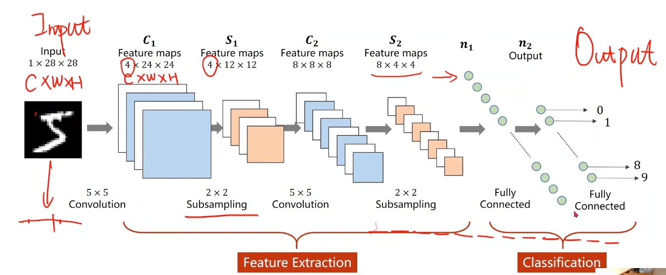
CNN Convolutional Neutral Network
-
Input: 1 * 28 * 28 的张量(channel * w * h)
-
通过一个卷积层 Convolution(5*5)(作用是保留图像的空间特征)
-
可以卷积成4 * 24 * 24(怎么卷的暂且不管,只要知道channel, w, h都可以变)
-
然后经过一个下采样(2*2)减少元素的数量(改变w, h,不改变 channel 数)
-
然后重复卷积+下采样,最终输出一个 1 阶的向量
-
最终映射成分类个数的维度,成为分类器
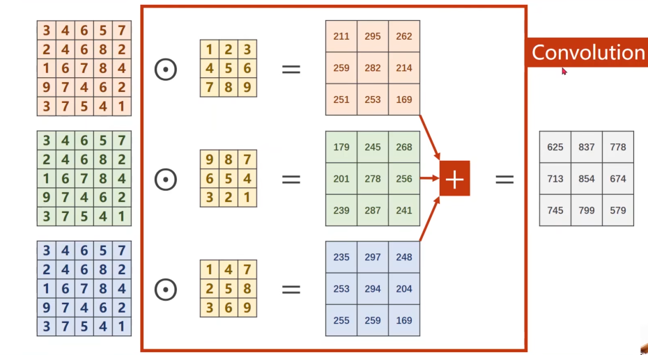
卷积层中,一个通道就要对应一个核(kernel)